A new measure of the impact of conflict on civilians
How are people affected by conflict?
ACLED and WorldPop have developed a tool that sheds light on this question, by providing information on the demographic and geographic characteristics of populations affected by conflict.
The Conflict Exposure Calculator integrates event-based conflict data from ACLED with population size estimates from WorldPop, to estimate the civilian impact by proximity to an event, event type, type of violent actor or specific armed group, location, and time.
Registered ACLED users can also see this exposure information in the dataset.
For more details on how to access this information in the dataset, see the relevant section below.
Overview
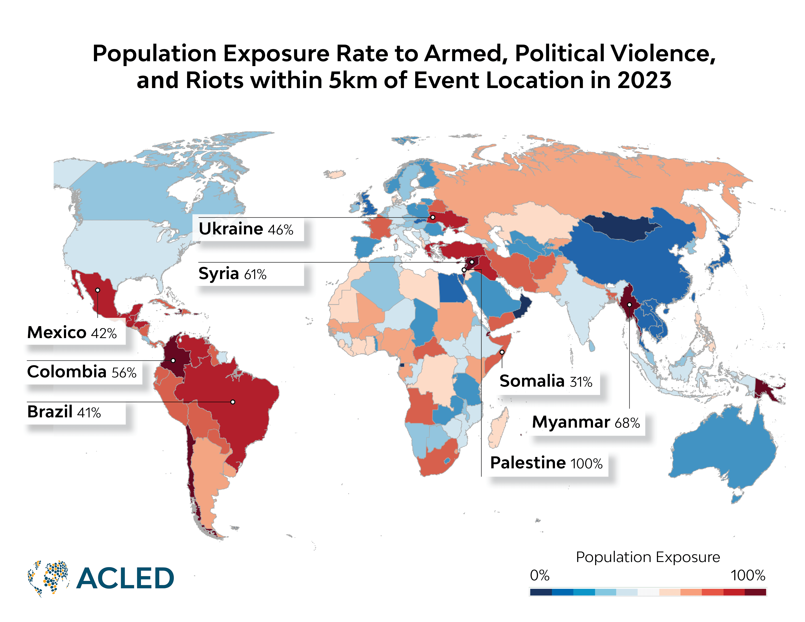
‘Conflict exposure’ is a measure of the number of people living within 1 kilometer, 2 km, and 5 km of each conflict incident or demonstration. Using this measure, we find that an estimated 14% of people in the world were within 5 kilometers of violent conflict in 2023.
To be exposed to conflict means that the population is living in an area of active disorder or unrest. People are harmed by this exposure in different ways: they may be directly injured; they may find themselves in active conflict; they and their group may be targeted; or they may be affected by the destruction of their village, neighborhood, or town.
This conflict exposure measure is the result of a partnership between ACLED and WorldPop.1Andrew J. Tatem, ’WorldPop, open data for spatial demography,’ Scientific Data, 31 January 2017 WorldPop produces fine-resolution population size estimates using remote sensing data to downscale national census information. Its integration with ACLED creates a population estimate of those close to violence; an estimate based on the most available demographic data. These data are extrapolations from census, remote sensing, and other information, but they are not updated with migration information, refugee flows, or IDP movements common in conflict areas.
Exposure levels can be calculated by incident, location, time, armed group, and group type, or can be aggregated to observe national and global trends. These data are available over time, and trends in exposure can be tracked.
Globally, conflict exposure is rising as more locations experience conflict (see the ACLED Conflict Index). Significant shares of the population in highly conflict-affected countries live near frequent and deadly conflict. Populations exposed to pronounced and repeated conflict risks are distributed widely at a global level. Because of the severe increase in conflict over the past five years, exposure rates to all forms of disorder and demonstrations have increased. In 2023, the average rate of conflict exposure across countries was 16%2At a 5 km buffer. but varied across countries (see Figure 1).
Conflict Exposure Measures
People living in conflict areas are not equally affected by conflict. Locations are differently exposed to violence, and armed groups use alternative strategies to advance conflicts that have an adverse effect on communities. Using the conflict exposure measure, it is possible to know the civilian impact by proximity to an incident by type of incident, by armed group and type of armed group, by time, by location, administration, or country, and globally.
What can this measure be used for?
People are exposed to conflict when it occurs in their geographic proximity. Population exposure statistics complement more typical conflict indicators, including incident or ‘event’ counts (measuring form and frequency), fatality summaries (a measure of intensity), or number of locations affected. ‘Exposure’ describes the outcome and extent of harm of these conflict events where the unit is an ‘estimated number of exposed people’ to those events in that location during a specific time period. Consider the example in Figure 2 in the Sahel from 2020-23, where conflict exposure is juxtaposed with conflict event frequency. Using both parameters, we see how intensely high rates of conflict due to competition between armed groups in the border regions of these three countries have exposed the same communities many times over to relentless violence.
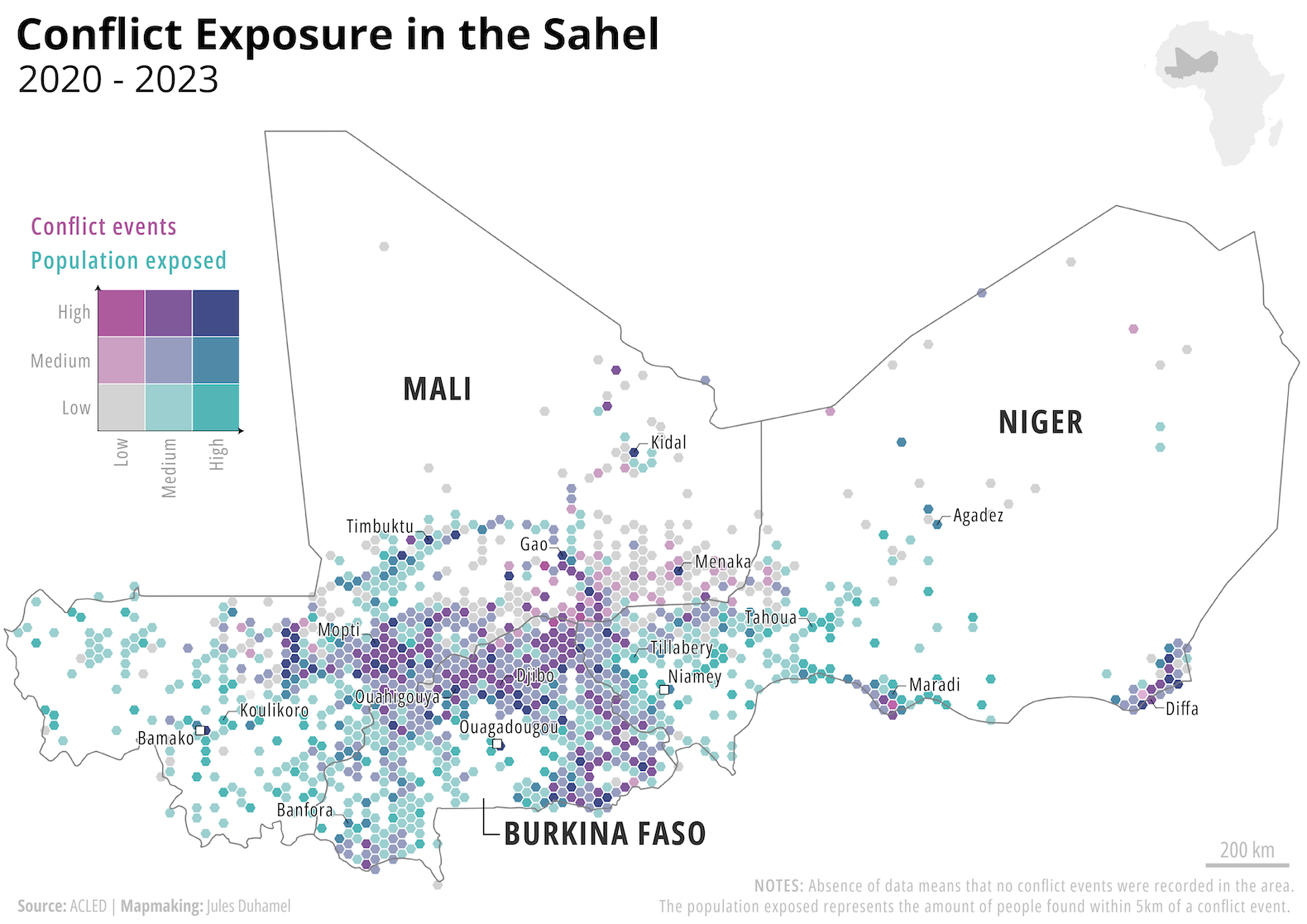
Figure 2: Conflict Exposure and Conflict Frequency Rates Across the Sahel 2020-23.
Conflict exposure measures tell us the demographic and geographic characteristics of populations affected by conflict. Almost all countries experience some form of political violence. However, we know little about the size and characteristics of populations exposed to violent incidents within those countries, despite significant advances in conflict research using event-level data,3Clionadh Raleigh, Roudabeh Kishi, and Andrew Linke, ‘Political instability patterns are obscured by conflict dataset scope conditions, sources, and coding choices,’ Humanities and Social Sciences Communications Journal, 25 February 2023 practitioner assessments of ‘population in need’ within violent environments,4Mine Action AoR – Global Protection Cluster, ‘What in People in need (PiN) and How do I calculate it?,’ accessed on 24 January 2024 and attempts to ascertain the economic ‘cost’ of conflict.5Anke Hoeffler, ‘What are the costs of violence?,’ Politics, Philosophy & Economics Journal,’ 13 July 2017 Conflict exposure measures can address several important questions, including:
- How many people are exposed to conflict?
- How many people are exposed to different forms of conflict? Who is exposed to conflict?
- Where and how many people are repeatedly exposed to conflict?
| Geographic Exposure | Demographic Exposure | Exposure Trends | |
|---|---|---|---|
| Addresses which question? | Where is exposed to conflict? | Who is exposed to conflict? | What are the exposure trends? |
| Assessment, Significance and Example | This dimension suggests patterns, strategies and variations of civilian exposure using maps, graphs, proportional location sizes and statistics | This assessment of risk reveals unequal and unseen exposure of civilians and its legacy through conflict exposure pyramids | This evaluation of trends and differences shows where and how risks to civilians are pooling and growing in global or national statistics, graphs and maps |
How accurate is conflict exposure data?
These measures of the civilian population living in areas affected by conflict or demonstrations are estimates. These estimates are based on a set of assumptions about the likely impact of those living proximate to conflict and demonstrations, and they are subject to other estimations, including the location of an event, and the best globally referenced method for estimating population. At present, these are annual, extrapolated estimates, subject to a calculation procedure that is designed to minimize population aggregation and possible exaggeration. Updates to locations used for ‘events’ in the ACLED dataset occur continuously; significant changes to WorldPop estimates are projected to be available in mid-2024. However, continuous efforts to estimate and integrate important population flows, including refugee and IDP movements, are ongoing.
What are the most important caveats and considerations when using these data?
Conflict exposure data measure the dispersed and concentrated outcome of events as ‘people exposed’ and is designed to limit over-aggregating exposed populations. The exposure measure will increase by year (or another observed time period), if people in new locations are exposed to violence or a demonstration. For example, if 100,000 people are living in the city of Nyala in Darfur and that city is attacked 15 times in one month, the conflict exposed number will remain 100,000 per month (rather than 1.5 million people). If Nyala is attacked 10 times in June and 10 times in July, and an analyst wishes to know the exposed population during each month, the conflict exposure measure will tell them that 100,000 people were exposed to conflict each month. It should only change if a new location and population are exposed, or if a new time period begins.
The conflict exposure measures need to be carefully calibrated by location and specific time period to avoid resulting in implausible aggregations. When using these raw data, calculate the exposure rate by location (e.g. global, country, town, etc.) and time period (year, month, day), and divide by the number of events that occurred in that location during that time period. This will provide the base assessment.
Further, because conflict exposure measures are specifically designed to limit over-aggregation, the extent of the buffers are for 1 km, 2 km, or 5 km, but the adjusted size is likely much smaller for areas with many conflict events and locations. For example, if in the city of Aden in Yemen, there are 50 locations that had at least one event in a year, and even 1 km buffers will overlap with neighboring buffers (as will 2 km and 5 km buffers). To prevent this, all buffers are designed to not overlap with any neighboring buffer. This results in a smaller unit than 1 km, 2 km, or 5 km as the area in which to assess the exposed population.
How does the ‘best’ estimate vary?
For each event in the ACLED dataset from 2020 onwards, the 1, 2, and 5 km estimates for each location and year are adjusted to create a unique ‘best’ conflict exposure estimate.
ACLED includes a ‘best’ estimate of conflict-exposed populations based on our knowledge of the impact and intensity of different ACLED ‘event types’. We base the ‘best’ estimate solely on a general rule for ‘event types’ and whether at least one fatality occurred. The default measures that comprise the best estimate are:
| Event types | Default measures |
|---|---|
| Battles | 5 km |
| Explosions/Remote violence | 5 km |
| Violence against civilians with no reported fatality | 2 km |
| Violence against civilians with at least one reported fatality | 5 km |
| Riots | 2 km |
| Strategic developments | N/A |
When summarizing the conflict-exposed population, the ‘best’ estimate will vary based on if that location has number of different ‘event types’. For more information on ACLED ‘event types’ and how events are recorded in the dataset see the ACLED Codebook.
How can you access conflict exposure measures?
Conflict exposure measures can be accessed in three ways.
The first is through the data portal. Once all data filters are complete, please note at the final step that conflict-exposed population measures need to be selected. There are two options for adding population data to the exported file: the default is to include only the ‘population_best’ column, providing the best estimate of exposed population, but users can also choose to download all four population columns with data on the different buffer sizes. That resulting file will include four columns called:
- Population_1km
- Population_2km
- Population_5km
- Population_best
The second way to access conflict exposure information is by downloading it via the ACLED API. The ‘population’ parameter allows for downloading either just the population_best column or all four population columns. See the ACLED API Guide for more details.
All registered ACLED users will have the same level of access to the conflict exposure data as they would to ACLED’s broader dataset. Please reach out to ACLED’s Access Team ([email protected]) if they require extended access.
The third way to access conflict exposure information is by using the Conflict Exposure Calculator. Using the calculator does not require downloading the data or registration.
What is the conflict exposure calculator?
The calculator is a tool that provides the most direct estimate of the exposed population for a given spatial unit (e.g. country/administrative region/town) during a specific time period (year, month, date) and can also vary by ‘event type’ and conflict actor.
How does the calculator aggregate population estimates?
The calculator summarizes population conflict exposure estimates based on applied filters, including spatial, temporal, interactions, armed groups or targeted groups, and/or ‘event types’. When there are multiple ‘event types’ for a location, the calculator applies the ‘best’ population estimate from the modal event type. This ensures that the ‘best’ estimate is the one associated with the most frequently occurring event type for each location. For example, if there was 1 ‘Battle’ event at a location (which defaults to the 5 km population estimate) and 10 ‘Violence against civilians’ events with no reported fatality (defaults to the 2 km population estimate) at that same location, the calculator applies the 2 km population option as the ‘best’ estimate, since this is the modal event type for the location.
If dates are selected in the calculator that span multiple years, the tool uses a weighted mean to account for different baseline population estimates for each ‘location-year.’ The calculator weights by the number of events that occurred within each selected year. For example, if 2022 and 2023 are selected, and there were 5 events in 2022 and 1 event in 2023 for a location, the estimate will weigh the 2022 population estimate five times more than the 2023 estimate. If the population estimate in 2022 and 2023 were 50,000 and 60,000, respectively, the weighted mean would be approximately 51,667.
Conflict exposure estimates may be viewed at varying levels of spatial granularity (location, first administrative level, country, or global). When aggregating above locations, the calculator sums the location-level estimates after accounting for modal event types and multiple-year rules above. When viewing the country-level results, the calculator shows the percentage of each selected country’s total population exposed to conflict, given the selected parameters and time periods. For the global results, the percentage of global population exposed estimate is calculated as the global exposed population given the menu selections relative to the summed population for countries that experienced at least 1 event, also given the selected parameters and time periods.
How often will conflict exposure estimates be updated?
ACLED data are updated weekly. For new locations added during the update, a revised population estimate at 1, 2, and 5 km is generated. If the 1, 2, or 5 km buffer of a new location overlaps with an existing location, the population estimate for the existing location will also be updated to prevent over-aggregation. For WorldPop updates, please refer to updates in the methodology section.
How do you cite conflict exposure measures?
Please refer to: ACLED data-conflict exposure. Date. Specific filters used.
Referring to the methodology or the concept, please cite:
Raleigh, C; C Dowd; A Tatem; A Linke; N Tejedor-Garavito; M Bondarenko and K Kishi. 2023. Assessing and Mapping Global and Local Conflict Exposure. Working Paper.
Methodology
Estimates of the size of the exposed population vary by the proximity boundary set around the location of the event. ACLED makes available estimates of the population living within 1 km, 2 km, and 5 km. Estimates of the exposed population for every new event are released along with the real-time weekly data from ACLED. A ‘best’ estimate can also be generated, which changes the boundary distance based on the type and intensity of the event. For example, for each explosion event, the ‘best’ estimate of the population exposed is set at 5 km encircling the specific location; however, the ‘best’ estimate for those exposed to a protest is 1 km. See the “How does the ‘best’ estimate vary?” question for more details on the ‘best’ exposure estimation.
ACLED and WorldPop Global Population Data
WorldPop is an applied research group at the University of Southampton, United Kingdom. The group produces many different types of small-area population estimate datasets to meet a wide range of needs and applications. These often involve different trade-offs in modeling methods and input datasets. This document briefly describes the datasets used in constructing the conflict exposure metrics, their limitations, and ongoing efforts to improve and update them. For further details, please see the WorldPop website, this overview paper, and available webinars on the production of population estimates and for emergency response.
To develop estimates of population numbers exposed to conflicts for all countries over multiple years, a globally consistent multi-temporal dataset provided estimated numbers of resident people in grid cells. These cells were then spatially linked with ACLED event-based conflict data. WorldPop’s global annual age/sex-structured population estimates for 2020-22 are used, and extrapolated.
Constructing a consistent multi-year time series of smal area population estimates across the globe requires a range of methodological assumptions and data trade-offs. Estimates are unlikely to be highly accurate compared to those purposely built for just a single, recent time point, or a single country. Nevertheless, the global datasets represent the best available current option from the WorldPop library, with updates and improvements coming soon (see below).
How WorldPop data are built?
The WorldPop global 2020-22 datasets are built through ‘top-down’ disaggregation modeling of a database of administrative unit-linked population estimates derived from subnational censuses and projections, constructed by CIESIN at Columbia University, and which primarily include censuses from the 2000 and 2010 rounds. Machine learning methods are used to construct models of the relationships between administrative unit-based population densities and a harmonized library of high spatial resolution gridded covariate data layers. This library and the modeled relationships are then used to disaggregate the administrative unit-based population counts to predictions of numbers of people residing in each 100×100 meter or 1×1 kilometer grid square globally. Further, an assembly of subnational demographic datasets are then used to break down these population totals by sex and age classes. Finally, national population totals are adjusted to ensure they match United Nations World Population Prospects estimates.
When calculating populations exposed to conflict using the WorldPop data, the following two-step approach is applied:
Creating Buffer Zones Around Conflict Locations:
First, a circular ‘buffer zones’ is drawn around each conflict location. These buffers can vary in size, typically set at 1 km, 2 km, or 5 km radii. However, in areas with multiple conflicts, these circles might overlap, leading to an overestimation of the population affected by the listed conflicts when they are added up, double-counting people. To address this, we use a technique called Voronoi tessellation.
When a set of points (representing conflict locations) is placed on a two-dimensional plane, Voronoi tessellation divides the plane into several polygons or cells, ensuring that each cell contains exactly one of these points. The boundaries of each cell are formed by the perpendicular bisectors of the lines connecting the central point to its neighbors. This effectively means each Voronoi cell is associated with a particular point and defines the area nearest to it. This characteristic makes Voronoi tessellation a preferred tool to delineate regions.
In areas with a high density of conflicts, the resulting Voronoi cells can be quite small, while in regions where conflict points are more dispersed, cells can be larger. To address this variance and achieve a more consistent representation of influence zones, we compute the geometric intersections between the Voronoi cells and the circular buffers initially created (see Figure 1). This combined approach allows for a more accurate and nuanced estimation of populations exposed to conflicts in varying geographic locations.
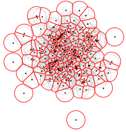
Figure 1. The constructed regions of influence (red) that are the intersection between the initial circular buffers (grey) and Voronoi cells associated withto the conflict locations.
Zonal Statistics to Extract Population Data
The ‘zonal statistics’ operation involves extracting the population data from the grid cells within the zones as determined in the previous steps. All cells with centroids falling inside the zones become the subject of the statistics. Since our primary interest is in the total population exposed, we aggregate the population counts within these zones.
The actual geometry of the buffer zones might be complex or disproportionate to the size of the grid cells. This mismatch means that the grid cells inside the zones may not perfectly align with the defined geometry (see Figure 2 below). To account for this discrepancy, an adjustment is necessary to refine our population estimate.

Figure 2. Illustration of the buffer zone (black polygon) around a conflict location (black dot) used to aggregate the population count from the gridded dataset (rectangular grids). Two cells are identified as being inside the zone.
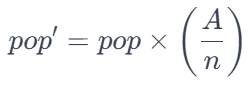
Consider the following: a buffer zone encompasses an area A (in km2) and contains n number of grid cells (each cell is 1 km2). If pop is the initial population count derived from the sum of these cells, we adjust it to better reflect the actual population within the buffer zone. The adjusted population count, pop’, is calculated as follows:
By applying these methods, we ensure a more precise estimation of the population exposed to conflicts, taking into account both the specific locations of these conflicts and the intricate geometries of the affected zones.
In constructing the population estimates used for the conflict exposure measures, choices are made based on needs and logistic limitations. To create ‘conflict exposure,’ the following choices are made:
- The ‘constrained’ dataset is used. WorldPop global datasets are available with either mapped populations constrained to satellite-defined settlement boundaries, or with predictions made for all grid cells. The difference is described here. Constrained data are found to be more accurate and appropriate for many global applications, and especially so for African countries where recent building footprint data were available to use.
- Interim 2021 and 2022 global datasets were constructed through simple adjustments of 2020 national population totals to match those in the UN World Population Prospects. The WorldPop global time series dataset was constructed for each year 2000-20 through a project funded by the Bill and Melinda Gates Foundation. WorldPop is in the process of producing a new and improved time series to cover the 2015-2030 period through a new project (see below), and these are expected to be ready in mid-2024 (see more below on ‘updates’).
- To enable the efficient calculation and rapid updates of exposure estimates, the 1 km spatial resolution global datasets were used, rather than the 100 m resolution data.
- Conflict often results in population displacement and migration and these are likely not captured in many settings due to the process of top-down disaggregation of census and projection data. WorldPop is engaged in multiple projects and activities to develop small-area population estimates that account for and update distributions when population movements occur. These include, for example, the integration of displacement survey and refugee camp data in South Sudan, disaggregating Common Operational Datasets on Population Statistics with UNFPA, the use of humanitarian datasets in Yemen, and estimating population baseline and change distributions in Ukraine. At present, none of these efforts and resulting datasets are currently included, and therefore uncertainties in exposure measures will be especially high where large-scale displacements have taken place. We aim to explore the integration of population estimates produced using methods that account for population movements in future work.
The effect of these trade-offs and methodological choices results in limitations to output estimates.
The extraction process described above has been implemented in a suite of Python scripts, which are publicly accessible on GitHub. These scripts are built upon a foundation of essential Python libraries, each serving a specific role in the analysis. For handling and manipulating large datasets efficiently, the scripts utilize NumPy and pandas. These libraries are fundamental for data analysis in Python, offering robust structures and functions for numerical and tabular data. The creation of circular buffers and the intricate process of clipping using Voronoi cells are handled using GeoPandas, SciPy-spatial, and Shapely. These packages provide comprehensive tools for geometric manipulations and spatial analysis. Finally, the rasterstats package is employed for the zonal statistics operation, enabling the extraction of population counts from gridded data within the defined zones.
A key feature of these scripts is their adaptability to dynamic conflict data. They are designed to allow for the easy integration of new conflict locations into the analysis pipeline. This means that when new conflict sites are added, the entire analysis does not need to be rerun from scratch. Instead, the scripts can update the population counts efficiently with the newly added locations. This flexibility ensures that the analysis remains current and can rapidly adapt to changing real-world situations, making it an invaluable tool for researchers and analysts monitoring conflict-affected populations.
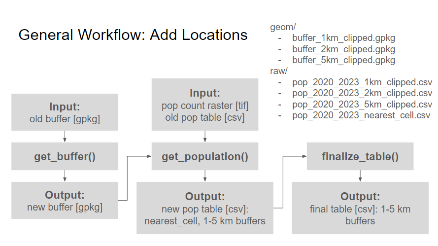
Figure 3. General workflow of extracting population exposed to conflicts at new locations.